
Implementing a Data Lakehouse Architecture in AWS — Part 3 of 4

Introduction
In our previous article, part 2 of the series, we walked through the extraction, processing, and creation of some data mart, using the New York City taxi trip data which is publicly available to do consumption. We used some of the principal technologies available for Data Analytics inside AWS, such as EMR, Athena, and Glue (Data Catalog and Schema Registry).
Now, we will show the processing steps using Tickit sample data provided by AWS in part 3. The processing phase takes the responsibility to bind the data with its object metastore and schemas provided by AWS Glue Data Catalog and Schema Registry respectively. By using Redshift Spectrum, we’ll be able to query processed data from S3, aggregate it and create some Data Mart inside Redshift.
Journey
Since the beginning of this blog series, we have discussed how each AWS resource will be created using terraform, from schemas and table metadata to the EMR cluster, processing the data and Redshift, using the Infrastructure as a Code (IaC) approach.
Below we will list each used resource and its role in that context.
Secrets Manager — Used to store the GitHub credential;
Amazon EMR — The managed Big Data platform for running large-scale distributed data processing jobs, leveraging the strategy to spend fewer computation costs using Spot instances. In this context, we will use it with Apache Spark;
Amazon S3 — We will use S3 buckets to store the data (extracted and processed);
Bucket: s3://dataeng-blog-series/ ;
Folder: raw/ (Receives the original data from Tickit samples provided by AWS.);
Folder: trusted/ (Contains the Tickit data with a well-defined schema after processing.);
AWS Glue Schema Registry — The repository to store and control the schemas and their versions for each object of our Data Lake;
AWS Glue Data Catalog — We will use the Glue Data Catalog to have a unified object metastore;
Amazon Redshift — makes it easier to run and scale analytics without having to manage a data warehouse infrastructure. Get insights running real-time and predictive analytics on all your data across your operational databases, data lake, data warehouse and thousands of third-party datasets.
The diagram below illustrates the proposed solution’s architectural design.

Proposed Environment
AWS Service Creation
To start the deployment we will validate the infrastructure code developed with Terraform.
If you don’t have Terraform installed, we will discuss two approaches in the solution below installing from the repository and downloading the standalone version.
# Installing from repository
$ curl -fsSL https://apt.releases.hashicorp.com/gpg | sudo apt-key add -
$ sudo apt-add-repository "deb [arch=amd64] https://apt.releases.hashicorp.com $(lsb_release -cs) main"
$ sudo apt-get update && sudo apt-get install terraform
$ terraform -version
Terraform v1.1.9
on linux_amd64


# Standalone version
$ curl -o terraform.zip https://releases.hashicorp.com/terraform/1.1.9/terraform_1.1.9_linux_amd64.zip && unzip terraform.zip
$ ./terraform -version
Terraform v1.1.9
on linux_amd64
Now, we need to initialize Terraform by running terraform init. This command will generate a directory named .terraform and download each module source declared in the main.tf file.
To validate the terraform code before the plan, use the helpful command terraform validate.
Following the best practices, always run the command terraform plan -out=redshift-stack-plan to review the output before starting creating or changing existing resources.
After getting the plan validated, it is possible to safely apply the changes by running terraform apply “redshift-stack-plan”. Terraform will do one last validation step and prompt confirmation before applying.
Data processing using Amazon EMR
By far, the most popular storage service for a Data Lakehouse is Amazon S3. Amazon EMR will allow you to store the data in Amazon S3 and run PySpark applications as you need to process that data. EMR clusters can be launched in minutes. We don’t have to worry about node provisioning, internal cluster setup, or other application/framework installation.
One of the most popular strategies used to achieve cost efficiency is the purchasing option of Spot instances, that in many cases could represent more than 60% of savings. This is according to the instance type and their availability within the selected AWS region.
Data Ingestion
The Tickit data provided by AWS is already available inside the RAW zone, where they were manually stored. Each table has its own format and is using a custom separator of columns. The table below describes each one.
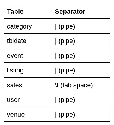 Table Separators
Data Processing — Trusted Zone
The second step of our data preparation process consists of fetching the data from the RAW zone, parsing the data by applying a new well-defined schema with the right data types for each column, and writing this data in parquet file format.
Below we have an example of a command processing the trusted zone.
# To process trusted data.
spark-submit process_data.py -r "s3://wp-lakehouse/raw/" -t "s3://wp-lakehouse/trusted/"
In our architecture, we are leveraging the resources of AWS Glue. In this case, our tables will be created inside the AWS Glue Data Catalog by receiving the schema definition from AWS Glue Schema Registry.
Here we could see the schema of all tables that were previously processed.
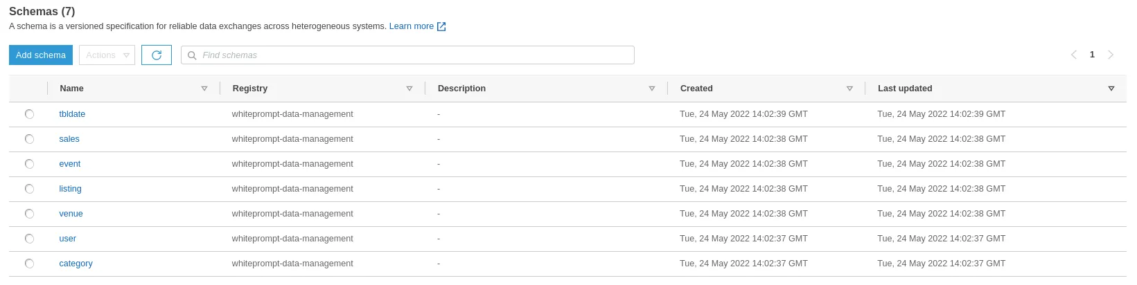 AWS Glue Schemas
The list of tables is available inside of the database wp_trusted_redshift by receiving its definition from the schema registry.
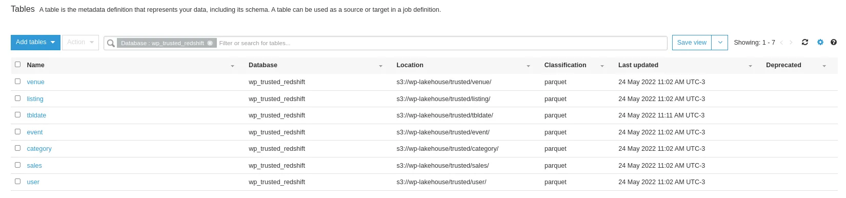 Glue Data Catalog tables
Redshift Spectrum — External tables from S3
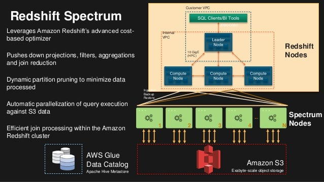
Amazon Redshift is a data warehouse service in the cloud. It was built to deliver a massively parallel processing solution that enables a cloud data warehouse for large-scale data sets solutions. For our deployment, we will use the Amazon Redshift Spectrum, which is serverless and will not require any additional resources to provision or manage.
By using Redshift Spectrum, we leverage the power of its processing engine to query data directly from S3 using standard SQL without the need for ETL processing.
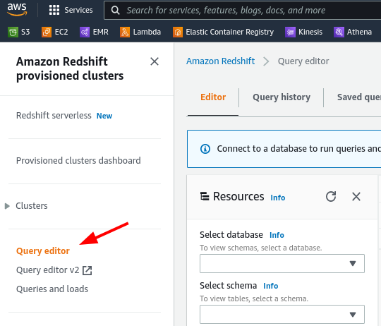
After the provisioning of our Redshift Cluster, we can see every cluster detail by looking at the console. We can use the JDBC or ODBC URL provided to connect from some external SQL client, but for this scenario, we will use the Query Editor directly from the Management Console.
With the active Redshift connection, open a new query and execute the command below to create the external schema referencing the Glue Data Catalog database.
CREATE EXTERNAL SCHEMA poc_spectrum FROM DATA CATALOG
DATABASE 'trusted_redshift'
IAM_ROLE 'arn:aws:iam::ACCOUNT_ID:role/lakehouse-spectrum-poc-redshift-role'
Since we had the data processing using EMR, our table metadata will be automatically available to Redshift.
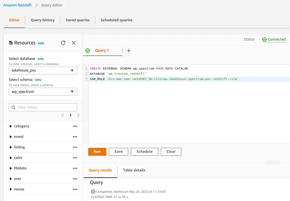 External schema creation
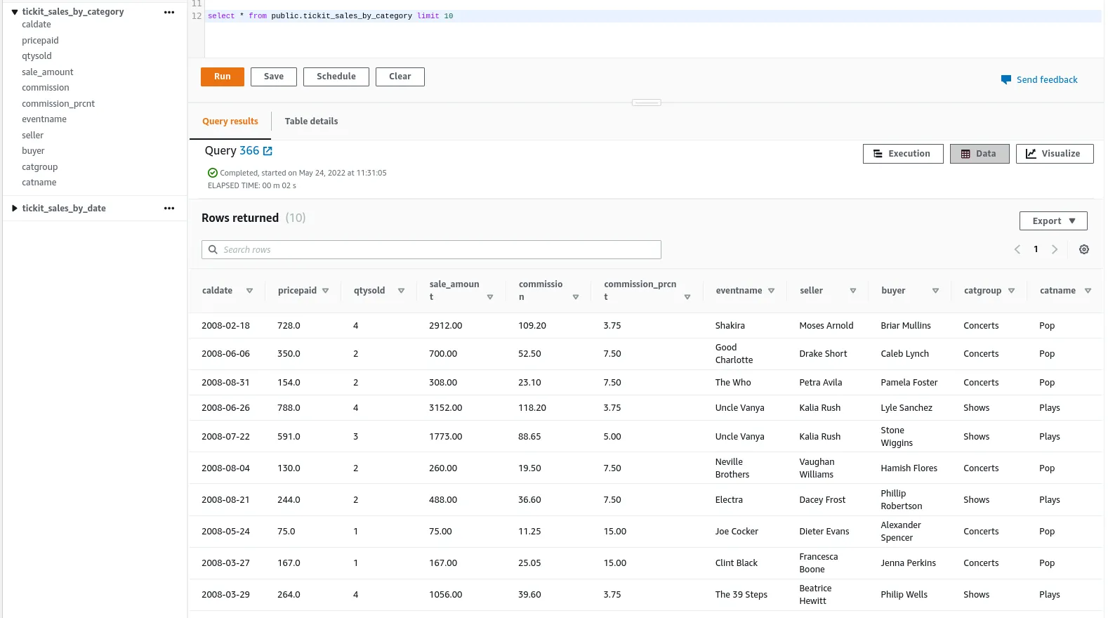
Now that we have all tables available inside of the Redshift, we will be able to create the Data Marts as public inside the schema by executing the commands below.
Data Mart: tickit_sales_by_category
CREATE TABLE public.tickit_sales_by_category AS (WITH cat AS (
        SELECT DISTINCT e.eventid,
            c.catgroup,
            c.catname
        FROM poc_spectrum.event AS e
            LEFT JOIN poc_spectrum.category AS c ON c.catid = e.catid
    )
    SELECT cast(d.caldate AS DATE) AS caldate,
        s.pricepaid,
        s.qtysold,
        round(cast(s.pricepaid AS DECIMAL(8,2)) * s.qtysold, 2) AS sale_amount,
        cast(s.commission AS DECIMAL(8,2)) AS commission,
        round((cast(s.commission AS DECIMAL(8,2)) / (cast(s.pricepaid AS DECIMAL(8,2)) * s.qtysold)) * 100, 2) AS commission_prcnt,
        e.eventname,
        u1.firstname || ' ' || u1.lastname AS seller,
        u2.firstname || ' ' || u2.lastname AS buyer,
        c.catgroup,
        c.catname
    FROM poc_spectrum.sales AS s
        LEFT JOIN poc_spectrum.listing AS l ON l.listid = s.listid
        LEFT JOIN poc_spectrum.user AS u1 ON u1.userid = s.sellerid
        LEFT JOIN poc_spectrum.user AS u2 ON u2.userid = s.buyerid
        LEFT JOIN poc_spectrum.event AS e ON e.eventid = s.eventid
        LEFT JOIN poc_spectrum.tbldate AS d ON d.dateid = s.dateid
        LEFT JOIN cat AS c ON c.eventid = s.eventid)
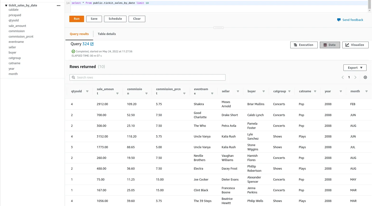
Data Mart: tickit_sales_by_date
CREATE TABLE public.tickit_sales_by_date AS (WITH cat AS (
        SELECT DISTINCT e.eventid,
            c.catgroup,
            c.catname
        FROM poc_spectrum.event AS e
            LEFT JOIN poc_spectrum.category AS c ON c.catid = e.catid
    )
    SELECT cast(d.caldate AS DATE) AS caldate,
        s.pricepaid,
        s.qtysold,
        round(cast(s.pricepaid AS DECIMAL(8,2)) * s.qtysold, 2) AS sale_amount,
        cast(s.commission AS DECIMAL(8,2)) AS commission,
        round((cast(s.commission AS DECIMAL(8,2)) / (cast(s.pricepaid AS DECIMAL(8,2)) * s.qtysold)) * 100, 2) AS commission_prcnt,
        e.eventname,
        u1.firstname || ' ' || u1.lastname AS seller,
        u2.firstname || ' ' || u2.lastname AS buyer,
        c.catgroup,
        c.catname,
        d.year,
        d.month
    FROM poc_spectrum.sales AS s
        LEFT JOIN poc_spectrum.listing AS l ON l.listid = s.listid
        LEFT JOIN poc_spectrum.user AS u1 ON u1.userid = s.sellerid
        LEFT JOIN poc_spectrum.user AS u2 ON u2.userid = s.buyerid
        LEFT JOIN poc_spectrum.event AS e ON e.eventid = s.eventid
        LEFT JOIN poc_spectrum.tbldate AS d ON d.dateid = s.dateid
        LEFT JOIN cat AS c ON c.eventid = s.eventid)
Below you will see a simple query execution to retrieve the data from both data marts.
Data Mart: public.tickit_sales_by_category
Data Mart: public.tickit_sales_by_date
Conclusion
In part 3 of this blog series, we have created a scenario to show a possible way to take advantage of many AWS resources in Data Analytics. By using Redshift Spectrum, we don’t need to ingest the entire dataset from our sources. Instead, we use the S3 Bucket as the cheapest and most scalable object storage to help the growth process in the Data-Driven Journey. With this deployment and others, we always consider the best way possible to achieve the integration while being cost-efficient for the project’s needs.
The new paradigm of the Data Lakehouse Architecture is arriving to deliver more opportunities to businesses where now the ranges of technology, frameworks, and cost related to Cloud Platforms are more attractive than ever.
Repository with the code used in this post.